W-ology, or, some exactly solvable growth models

by Keith Briggs (formerly at Department of Plant Sciences, University of Cambridge, Downing St., Cambridge CB2 3EA. Revised 1999 Nov 12; font adjustments 2005 July 11)

`To give full growth to that which still doth grow?' - Shakespeare, Sonnet CXV

Introduction

Aim of these notes: to show how some generalizations of logistic growth laws have elegant analytic solutions and speculate on their applications to modelling.

Lambert's W function is defined by

Useful formulas

1. The solution of (a+bx)exp(cx)-d = 0 is

   x = W[cd/bexp(ac/b)]/c-a/b.

   Example application: in New Phytol. 136, 362 (1997), the equation (q₁+q₂ R)exp(-q₃R)-0.05 = 0 needed to be solved for the pathozone width R. This is trivial with the above formula: R = -W[-(q₃/(20q₂))exp(-q₁q₃/q₂)]/q₃-q₁/q₂. Similar transcendental algebraic equations arise in the computation of equilibria in graph-theoretical epidemic models.

2. W'(x) = W(x)/(x(1+W(x))) for x nonzero.
3. ∫ W(x)dx = x[W(x)-1+1/W(x)]+c

4. The inverse function W ^{< -1 >} is given by W ^{< -1 >} (x) = xexp(x).
5. The Taylor series of W around 0 is ∑_{k = 1}^∞[((-k)^k-1)/k!]x^k, and has radius of convergence e^-1.

Differential equations

It is usually considered that the most general exactly solvable growth model is that of Richards:

(ν not 0, ν> -2) for which the solution is

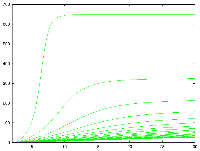
with J a function of Κ,ν and y(0).

Instead, I wish to consider models of the form

1. ∫[dx/(x(1-bx))] = log(x)-log(bx-1)
2. ∫[dx/(x²(1-bx))] = b(log(x)-log(bx-1))-x^-1
3. ∫integral[dx/(x³(1-bx))] = (-x^-2/2-bx^-1)-b²(log(bx-1)-log(x))

etc.

These allow us to give explicitly the solution of the initial value problem

Figure 1: Solutions of equation (4) for y₀ = 3,a = 0.001,b = 8,12,18,32,62

A very rough fit of equation (4) to some onion plant growth data is shown in Figure 2. No attempt has been made to optimize the parameters.

Another differential equation, which can be interpreted as having a time-dependent growth rate, is

Figure 3: The functions v(x) for various b

Lotka-Volterra models

The two-species model

Take-home message

A numerical algorithm for W

/* ANSI C code for W(x).  K M Briggs 98 Feb 12 
   http://www-epidem.plantsci.cam.ac.uk/~kbriggs/LambertW.c
   Based on Halley iteration.  Converges rapidly for all valid x. */
double W(const double x) {
  int i; double p,e,t,w,eps=4.0e-16; /* eps=desired precision */
  if (x<-0.36787944117144232159552377016146086) {
    fprintf(stderr,"x=%g is < -1/e, exiting.\n",x); exit(1); }
  if (0.0==x) return 0.0;
  /* get initial approximation for iteration... */
  if (x<1.0) { /* series near 0 */
    p=sqrt(2.0*(2.7182818284590452353602874713526625*x+1.0));
    w=-1.0+p-p*p/3.0+11.0/72.0*p*p*p;
  } else w=log(x); /* asymptotic */
  if (x>3.0) w-=log(w);
  for (i=0; i<20; i++) { /* Halley loop */
    e=exp(w); t=w*e-x;
    t/=e*(w+1.0)-0.5*(w+2.0)*t/(w+1.0); w-=t;
    if (fabs(t)<eps*(1.0+fabs(w))) return w; /* rel-abs error */
  } /* never gets here */
  fprintf(stderr,"No convergence at x=%g\n",x); exit(1);
}

Bibliography

I've tried to make these notes self-contained, so all you should need is...

[1] Briggs, K. M. W-ology, or, some exactly solvable growth models

Footnotes: